Diving Deep Into Quantum Computing: Computing With Quantum Mechanics
By Morton Swimmer, Mark Chimley, and Adam Tuaima
Quantum mechanics enables us to build computers that are, in some ways, much more powerful than classical computers. Small, gated quantum computers and experimental quantum computers already exist, but the world might soon see the arrival of quantum computers capable of demonstrating quantum advantage over their classical counterparts. When that happens, it will leave little time for the lengthy process of migrating to new cryptographic algorithms, so it’s best to plan ahead and consider post-quantum cryptography now.
In this entry, the second in our series on post-quantum cryptography, we delve into the history of quantum computing, its foundation in quantum mechanics, and the kind of complex problems quantum computers will be able to solve.
Brief history of computing
To better comprehend quantum mechanics, it helps to understand how mathematics evolved over time, and with it, our understanding of nature.
Early in history, people’s mathematical understanding of the world was simpler than now: at first, only natural numbers (1, 2, 3, 4, 5, etc.) were used to count. Later, negative numbers (…, -3, -2, -1, 0, 1, 2, 3, ….) were incorporated as well. Eventually, multiplication and division were needed, and these required the concept of fractions created from positive integers. These were classified as rational numbers.
Rational numbers serve well in many practical applications of physics or classical mechanics, where the goal is to measure or approximate something to a sufficient degree of accuracy. However, when the ancient Egyptians wanted to calculate the area of a circle, they tried using fractions in their formula, but the results were not quite accurate. Further examination revealed that a certain number, which will eventually be called pi (symbolized by π and has the value of 3.14159…), can instead be used for this operation. This sparked the idea that there are numbers that cannot be represented by fractions. We call such as real numbers because there’s a tacit assumption that they describe how nature works. So, for a long time, people believed that the world exists on a continuum of scales.
However, the advent of nuclear physics in the late 19th and early 20th centuries started to challenge this view. The smallest unit of matter was initially thought to be the atom, thus it was so named — the ancient Greek “atomos” translates to “indivisible,” or more literally “uncuttable.” In the late 19th century, however, Sir Joseph John Thompson discovered a sub-atomic particle, the electron, and proposed the ‘plum pudding’ model of an atom. In the early 20th century, Ernest Rutherford first theorized the existence of protons and neutrons in an atom’s nucleus, a fact then proven by James Chadwick. Rutherford proposed a model of the atom where the electrons orbited the nucleus like planets around the sun.
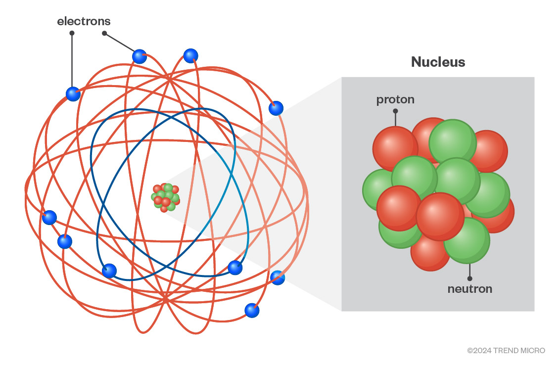
Figure 1. Rutherford Atomic Model
But trouble was on the horizon for the planetary model of an atom. Viewed through the lens of classical electromagnetic physics, the electrons would have to continuously lose energy and their orbits would decay rapidly, resulting in the collapse of the atom; but this was not happening.
Meanwhile, Albert Einstein proved Max Planck’s hypothesis that matter has both particle and wave characteristics, for which he later won the Nobel Prize. This is called the wave/particle duality. With this, Niels Bohr, one of the founding fathers of quantum theory, presented a superseding model of the atom in which electrons occupy a set of discrete (or quantized) positions (orbits) based on their energy levels. Describing each orbital by the wave function of the electron explains why the orbitals do not collapse: the smallest orbital is the one composed of a single standing wave. Electrons can move from one discrete state (quantum) to another, but they do so discontinuously; that is, they jump between quanta in a quantum leap. Each jump goes from one wave harmonic to another. The earlier assumption that the world is based on real numbers was proven incorrect. Wolfgang Ernst Pauli later determined that no two electrons can inhabit the same state at the same time, making the model useful in predicting an atom’s chemical properties.
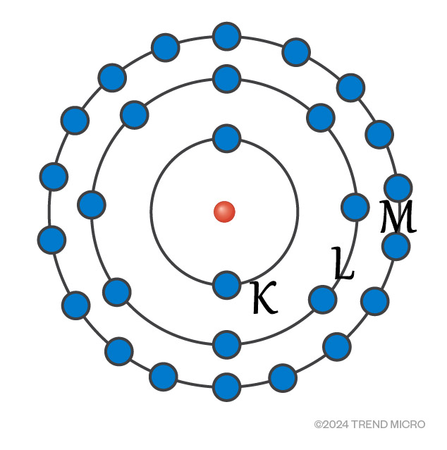
Figure 2. Bohr Model
Most of these might be hard to relate to everyday experiences, but they sit coherently within the quantum mechanical model in terms of mathematics. While many scientists in the early 20th century — for instance, Einstein — were skeptical of quantum mechanics, over time, the field has proven to be sound and useful.
Other observations that fit the quantum model include Heisenberg's uncertainty principle, which states that it is not possible to precisely determine both the momentum and position of an electron. The more accurately we discern one aspect (either momentum or position), the less accurately the other aspect is determined. This is not a limitation of the apparatus. This is a fundamental property of quantum mechanics and plays an important role in quantum computing.
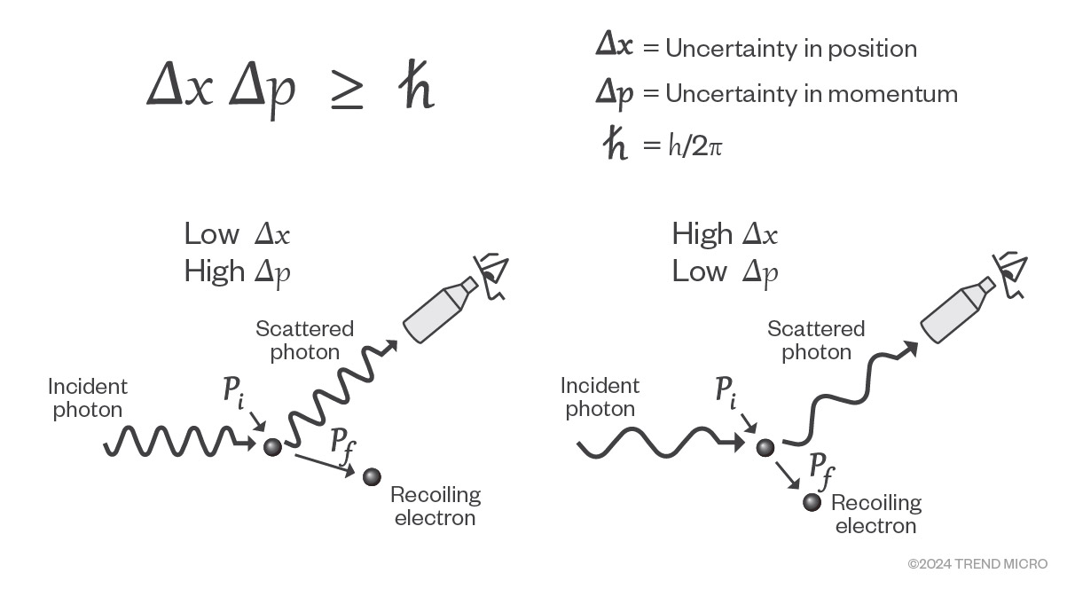
Figure 3. Heisenberg’s Uncertainty Principle
As shown in the left portion of the illustration above, if we use a high frequency to determine the location of an electron, we will not know its momentum with good accuracy. If we use a low frequency, we can find its momentum with good accuracy but will then not know its location well. In the quantum mechanical world, any measurement comes with a trade-off.
Heisenberg’s uncertainty principle changes how we think about computation. While in a classical computer, reading from a memory location doesn’t change it, the same is not true in a quantum computer. Reading the state of a quantum system will invalidate its state, so algorithms need to be designed appropriately.
Two other important topics in quantum mechanics are superposition and entanglement. These are central to quantum computing. Together, they make quantum computing possible.
Superposition
Until they are measured, particles can exist in infinitely many states. Take an electron, for instance. It is said that it can spin on the x, y, and z axes, as shown in Figure 4. When an electron’s spin is clockwise along some axis, we can call this the “1” state and when it is spinning counterclockwise, we call this the “0” state. However, before measuring the spin, the electron is in a superposition of all possible states. Think of a spinning coin: we cannot say it is in a heads or tails state while it is spinning. Rather, it is in some other in-between state. It’s in a superposition. (Note that the electron doesn’t actually spin. This is just a measurable property of it that we chose to call “spin”.)
The particle is in superposition while it is not observed. When the spin is measured, the state will “collapse” on one choice dictated by its probability distribution, just like when the coin flops down on one side or the other with a 50% chance of being either.
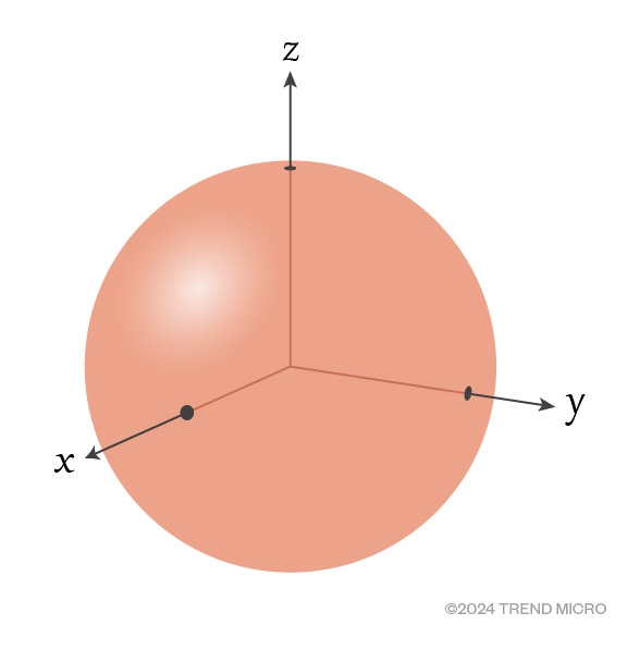
Figure 4. An electron can “spin” on the x, y, and z axes
This is the basis of the famous Schrödinger’s Cat thought experiment (Figure 5). An imaginary cat is placed in a box with a vial of poison and a radioactive source. If radioactive decay is detected, the vial of poison breaks and ends the imaginary cat’s life. But radioactive decay is a random process which may or may not happen.
While this was originally meant to demonstrate the absurdity of quantum mechanics, it turned out to be a reasonable explainer of superposition. When the box is shut, there is no way of observing what happens inside. Whether the cat is alive or dead cannot be concluded. From an observer’s point of view, the cat is in a superposition of dead and alive. In quantum mechanics, opening the box causes the superposition to collapse into a single state of the cat being either dead or alive.
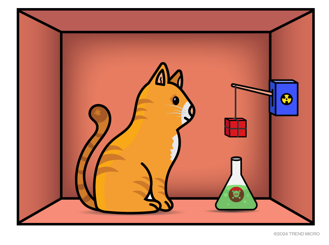
Figure 5. The Schrödinger’s Cat thought experiment
Qubits and quantum circuits
In a classical computer, the smallest unit of storage is called a bit, which can either take a 0 or a 1. In a quantum computer, particles can be used to perform calculations, and these are called qubits (quantum bits). Qubits are different from ordinary bits in that through superposition, they can assume an infinite number of states at the same time, which gives them exponentially more computational power. Qubits are used in quantum circuits, which are comparable to algorithms on a classical computer. The goal of these circuits is to run to the end and amplify the correct result so that the answers can be read by measuring the resulting states. In practice, the circuit is re-run thousands of times to obtain a probability distribution from which the answer is derived. However, a circuit needs gates, and the use of multiple gates requires entanglement. The following section delves into this concept.
Entanglement
In a classical computer, a logic gate can take bits as input and produce a value as output. For example, a “1” bit and another “1” bit combined at an AND gate will result in “1”. On their own, these bits do nothing. However, in a quantum computer, two particles can become “entangled,” which means an operation on one will influence the state of the other, even if they are far apart. This is like picturing two spinning coins that always land down the same way: either showing both heads or both tails. The two particles are not communicating with each other to do this. Instead, imagine them as twins that behave the same even when they are separated. In this way, they are not violating special relativity that disallows travel at the speed of light or faster. In the macro world, however, this would be strange, and we would not expect coins to behave this way.
Einstein was not a fan of the idea and described it as “spooky action at a distance.” It might take some convincing to believe that that two particles could influence each other remotely, but it is mathematically proven by and shown in experiments. Between 1980 and 1982, Alain Aspect performed various experiments proving entanglement is real, for which he won the Nobel Prize in 2022.
Entanglement makes useful algorithms possible. By linking two qubits, conditional quantum gates can be created in quantum circuits. With that, algorithms can be implemented.
Why quantum computers?
When the first serious efforts to build a quantum computer were made in the mid-1990s, one of the main questions raised was, what would it be good for? Actually, this very question serves as the answer itself to one of the main motivations why these computers are developed: they were built so their full potential can be discovered and unleashed.
The original idea of quantum computing was proposed by Paul Benioff and Richard P. Feynman around 1980. Simulations of physical systems, for instance tracking all interactions between atoms in a molecule, are often impossible to run on classical computers because the difficulty of the problem grows exponentially with the number of atoms. In contrast, quantum computers can tackle exponentially larger problems for every qubit in the quantum computer and can deal with this complexity.
Now, while experimental quantum computers are emerging, there are still challenges on how their usefulness can be most effectively maximized. Machines with sufficiently large numbers of usable qubits remain elusive. Furthermore, scalability and noise management remain a concern. Noise could limit scalability. In this context, noise pertains to electromagnetic radiation, magnetic fields, cosmic rays, and the like. For this reason, most quantum computers are operated at temperatures close to absolute zero (which is 0 Kelvin, -273.15℃, or -459.67 ℉) and are heavily shielded from radiation.
With the current crop of quantum computers, attempts to mitigate noise are done by using redundant noisy physical qubits to create noise-free logical qubits. The current generation of quantum computers is called Noisy Intermediate-Scale Quantum (NISQ) computers. The number of logical qubits is much lower than the number of physical qubits in these systems. This means that a useful quantum computer will have to have several dozen times as many physical qubits as required logical qubits in order to execute a given quantum circuit.
Despite the challenges, many algorithms for quantum computers have been proposed, showing how versatile the platform may one day be. As of now that question of their purpose still stands, although perhaps not much longer.
Quantum advantage
Quantum advantage pertains to the milestone where a quantum computer can solve problems faster than a classical computer can. While several claims of quantum advantage have been made recently, none of them solves useful problems. They are therefore not convincing — yet. Because the simulation of physical systems often requires far fewer qubits, we will probably see the first practical uses here. On the other hand, a quantum computer for solving large computer science problems is probably over a decade away. These simulations would be valuable as they would enable major chemical, physical, and medicinal discoveries. This is why the development of quantum computers has garnered so much attention lately.
In an attempt to horizontally scale the current generation of experimental quantum computers, there have been experiments using circuit knitting or surface-code architectures. These experiments take small quantum computers and combine them using classical or quantum connections to form a larger machine. However, it is not clear if quantum advantage can be achieved this way, as these separate circuits need to be connected, which incurs overhead and a change to the algorithms. The last limiting factor is the number of quantum gates that can be used, but little has been published on this for existing quantum computers.
Quantum computers in the real world
Small, gated quantum computers containing a few hundred physical qubits, are now available as a cloud service from various vendors. Adiabatic quantum computers (AQC) that are restricted to a special optimization process already have thousands of qubits but have yet to show meaningful speedup over classical computers.
A recent finding from a university in Switzerland showed that merely quadratic speedup over classical algorithms will not be enough to compensate for the overhead that quantum computers have in loading the data and circuit. Given this finding, there are some doubts that they will ever be useful for big-data applications at all, unless some engineering solution is found.
Quantum computer complexity classes
As mentioned, quantum computers can solve some problems in minutes that would take years on a classical computer. In this section, let’s look at the classes of problems that quantum computers can solve.
A complexity class refers to a set of problems that are solvable with relatable time requirements on a Turing machine, which is a theoretical computational model. Without going into details, a nondeterministic Turing machine is exponentially faster than the deterministic variant. We strive to use polynomial-time algorithms (or better) because the time they take only goes up moderately with the problem size. We call these “P” problems. Many real-world problems are “NP” problems that require much greater resources and typically grow in time and space requirements exponentially with the size of the input problem. We say that a problem is NP-Complete if it can be proven that no algorithm solves the problem better than a non-deterministic Turing machine would need in polynomial time. The entire space of decidable problems that a Turing machine can solve is called PSPACE.
The complexity class for quantum algorithms solvable in polynomial time is called Bounded-Error Quantum Polynomial Time complexity (BQP). This class is not thoroughly explored, but we believe it includes the whole P class and some of the NP and PSPACE classes, but no NP-Complete problems (as shown in Figure 6 below). Solving some of the NP problems in BQP time complexity is a game changer, even if it might disappoint some that NP-complete problems still stay exponentially difficult.
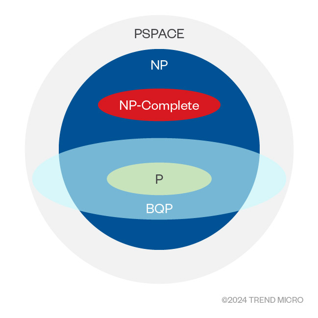
Figure 6. Quantum computer complexity classes
What quantum computers cannot do is solve completely intractable and (classically) undecidable problems. And while there are problems that are difficult for classical computers but relatively easy for quantum computers, the reverse is also true.
The rise in interest in quantum computing algorithms has also revived creativity in classical algorithm design. Some heuristic algorithms can now be seen emerging from this research. These are often optimization algorithms that are called Quantum Inspired Optimization (QIO) or sometimes Quantum-Inspired Algorithms (QIA). Therefore, research into quantum computing is leading to speedups in classical real-world algorithms, which might turn out to be more of a game changer than quantum computers themselves.
Conclusion
Quantum computers are vastly different from classical computers in fundamental ways. This is shown through a variety of factors, from the probabilistic nature of their operation to the resulting complexity classes of the algorithms that can be implemented on quantum computers. This article looked into the history of quantum computing, pertinent concepts in quantum mechanics, and the type of problems quantum computers can help solve. It also touched on the types of gates that can be used in quantum circuits. In the next parts of this research, we will look at how quantum computer cryptanalysis works and why there are worries about these nascent computers.
Like it? Add this infographic to your site:
1. Click on the box below. 2. Press Ctrl+A to select all. 3. Press Ctrl+C to copy. 4. Paste the code into your page (Ctrl+V).
Image will appear the same size as you see above.
- TrendAI™ 2026 Cyber Risk Report
- The Hidden Risk in Your AI Rollout: Your Endpoints
- When AI Becomes a Zero-Day Machine: What Public Sector Organizations Need to Know
- A Data-Driven View of Cyber Risk Structure: How Attack Pressure and Exposure Shape Damage
- Hunt Them All: An AI-Powered Vulnerability Sweep of 19,000 MCP Servers
 Fault Lines in the AI Ecosystem: TrendAI™ State of AI Security Report
 It’s By Design: The Use-After-Free of Azure Cloud
 TrendAI™ 2026 Cyber Risk Report
 Guarding LLMs With a Layered Prompt Injection Representation